Introduction
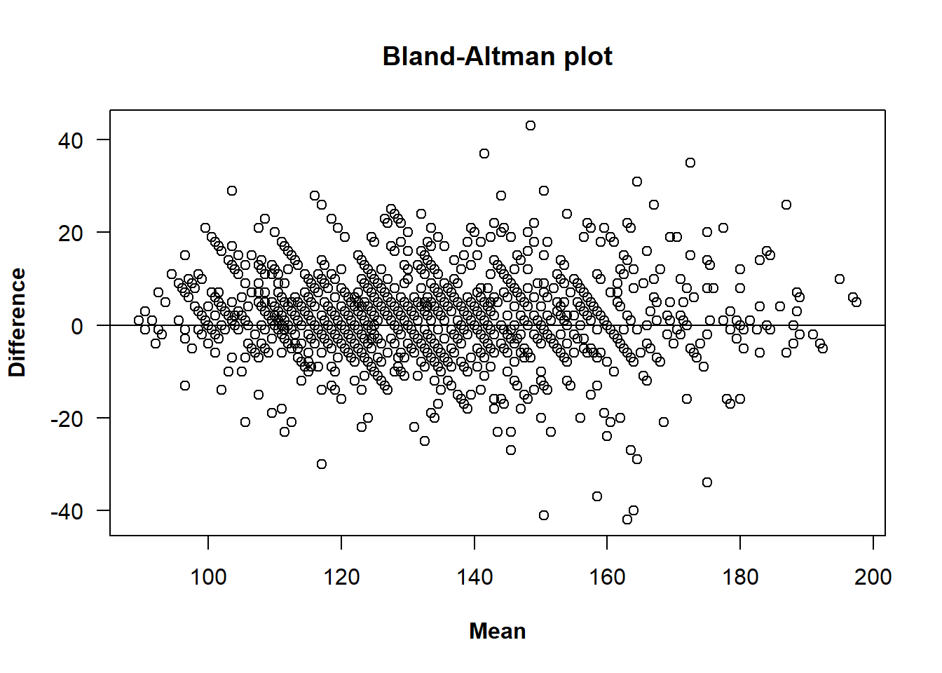
In the case of two raters, the most simple graphical approach to assess agreement is a scatterplot of the measurements obtained from one rater against those from the other. In this scatterplot, the bisector is the line of concordance in which all points lie in the case of perfect agreement. However, while the scatterplot is informative, it may fail to reveal certain types of disagreement, especially when measurements are strongly correlated. In order to address this issue, Bland and Altman (1986) suggested plotting the difference of the measurements taken by the two raters against their mean for each subject. In the case with replicates, all paired-differences and means are plotted. One of the advantages of this plot is that it might reflect between-rater differences that are not obvious from a simple scatterplot of the results of one rater against those of the other. In the Bland-Altman plot we can evaluate if the mean and the variance of the differences remain constant across the range of measurements. In particular, it facilitates the identification of systematic bias between raters and helps assess whether the extent of the disagreement between raters varies with the magnitude of the measurements, which is approximated by the mean of the two raters. This makes the Bland-Altman plot especially helpful for identifying trends such as systematic bias or heteroscedasticity.
To illustrate the use of the plot.tdi() method, it is
applied to the same sample dataset used in the vignettes for the
functions descriptive.plots()
and TDI().
We begin by loading the dataset and getting it ready for the analysis.
library(cccrm)
bp <- bpres[, c("ID", "SIS", "METODE", "NM")]
colnames(bp) <- c("id", "sys", "met", "rep")
bp[, c("id", "met", "rep")] <- lapply(bp[, c("id", "met", "rep")], as.factor)
Note: In this study we identified five measurements
in which the results from the two raters differ substantially. These
readings originated from three specific individuals whose identification
numbers were 24, 199 and 226. After discussions with clinical
practitioners, these discrepancies were attributed to transcription
errors (and not to the error introduced by the device itself). Since we
could not recover the correct values of these measurements, we decided
to discard all measurements from these patients. Consequently, the
filtered dataset is used for all subsequent analyses and examples in
this vignette. Eliminating these patients will leave empty levels in the
id column, causing warnings to appear in subsequent
function calls. While these warnings can be safely ignored, it is good
practice to clean up unused levels using droplevels()
before proceeding:
bp <- bp[!bp$id %in% c(24, 199, 226), ]
bp$id <- droplevels(bp$id)
The default call to the plot.tdi() method requires a
tdi object generated by the TDI() function.
Since the function relies on bootstrapping to estimate confidence
intervals in the method of Perez-Jaume and Carrasco, we set a random
seed beforehand using set.seed() to ensure exact
reproducibility of the plot:
General arguments that can be modified are main,
xlab, ylab, xlim and
ylim, with their well known meaning.
plot(x, main = "Blood pressure data",
     xlab = "Mean (mmHg)", ylab = "Difference (mmHg)",
     xlim = c(80, 200), ylim = c(-60, 60))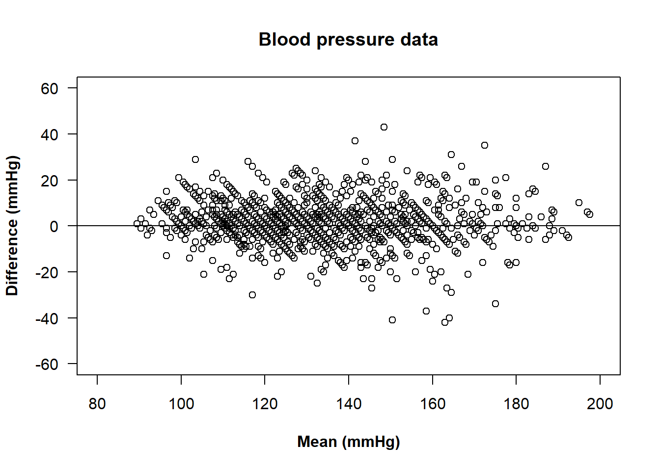
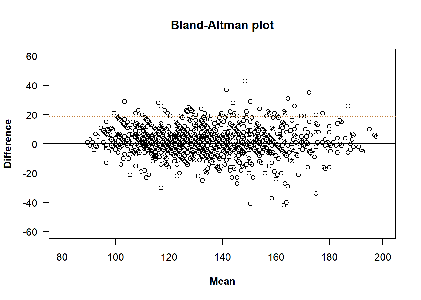
Bland and Altman also proposed to compute what they called ‘’limits of agreement’’ (LoA), which intended to predict an interval that contains most of the differences between raters. The limits of agreement are based on the assumption that the differences are normally distributed, which is not always the case, and are conditioned to the direction of the differences. The \(100(1-\alpha)\%\) LoA are defined as \[ \bar{d}\pm z_{1-\frac{\alpha}{2}}\cdot \text{sd}(d), \] where \(d\) represents the vector containing the paired-differences between both raters, \(\bar{d}\) represents their mean and \(\text{sd}(d)\) represents their standard deviation.
These values can be added to the Bland-Altman plot as horizontal
lines to assess agreement by evaluating their magnitude and their
clinical relevance. It can be done with the loa argument,
setting it to TRUE.
We can add a legend or change the colour of the lines.
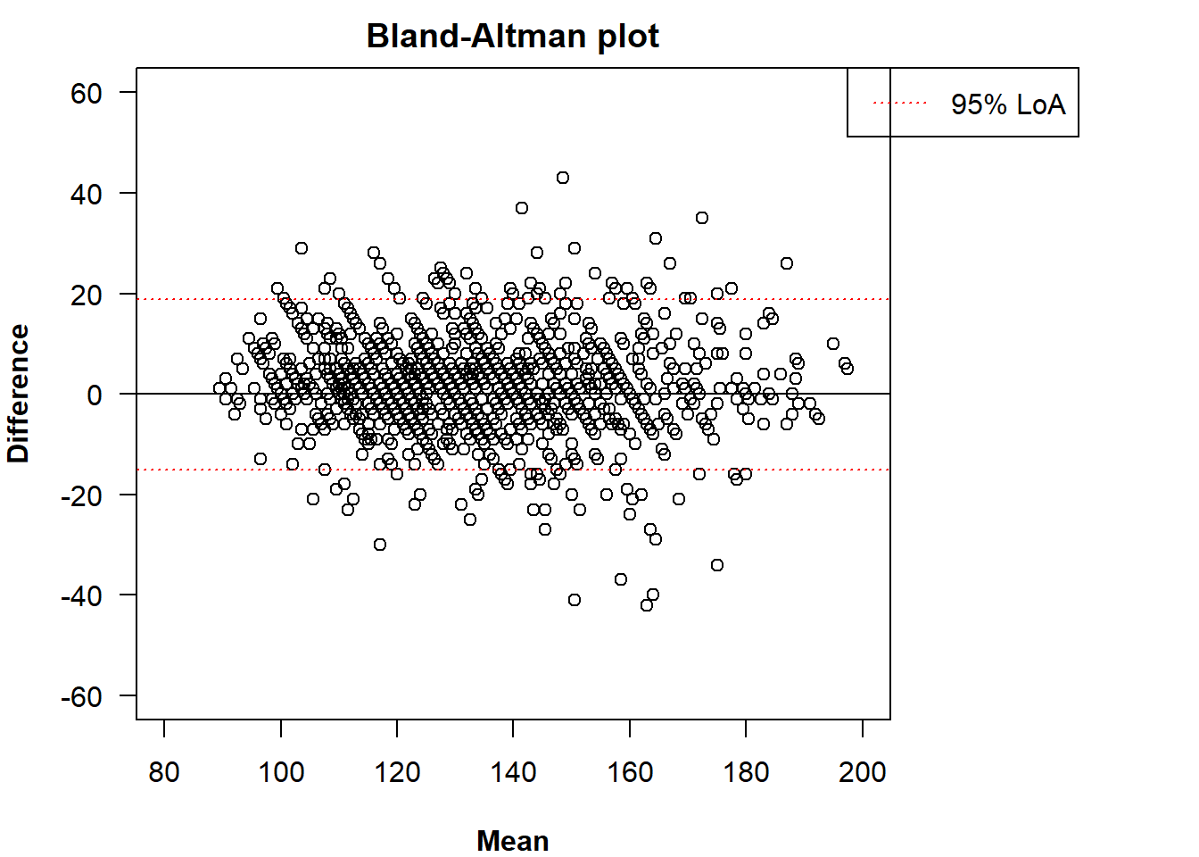
The legend can be adjusted with the inset argument
(passed to legend()).
plot(x, loa = TRUE, loa.col = "red",
     legend = TRUE, inset = c(-0.34, 0),
     xlim = c(80, 200), ylim = c(-60, 60))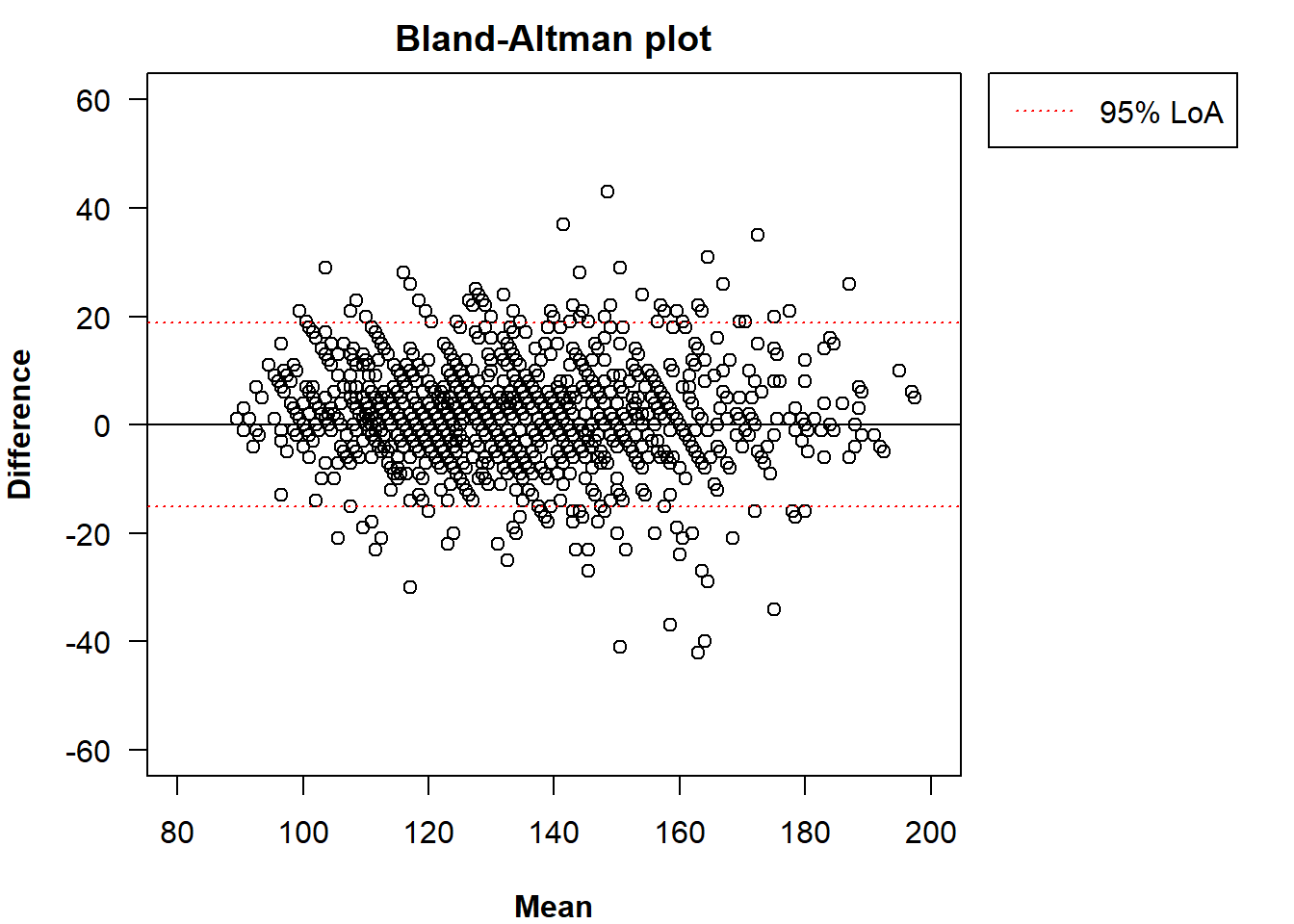
An alternative to the LoA is the TDI. Its estimate or its UB (and
their negative counterparts) can also be added to the Bland-Altman plot.
Unlike the LoA, which is centred around \(\bar{d}\), the interval \([-\hat{\text{TDI}},\hat{\text{TDI}}]\) is
centred around zero and considers the absolute magnitude of the
differences instead of their direction. We can add them with the
arguments tdi and ub.
plot(x, tdi = TRUE, ub = TRUE,
     legend = TRUE, inset = c(-0.4, 0),
     xlim = c(80, 200), ylim = c(-60, 60))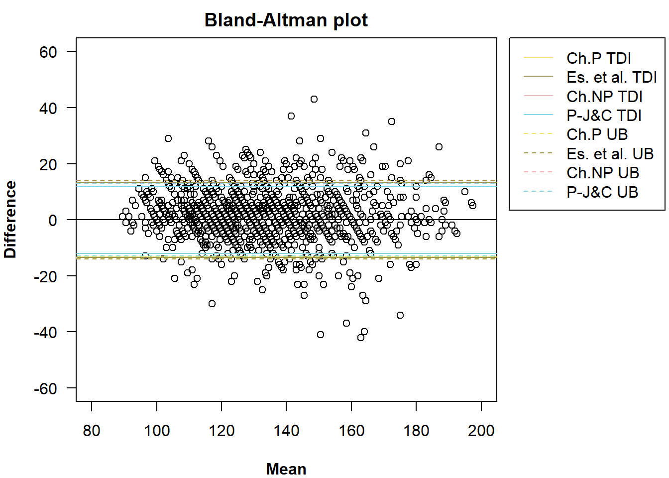
All estimated methods from the call of the function
TDI() are added by default. We can specify which one(s) we
want to add with the argument method.
plot(x, tdi = TRUE, ub = TRUE,
     method = c("es", "pe"),
     legend = TRUE, inset = c(-0.4, 0),
     xlim = c(80, 200), ylim = c(-60, 60))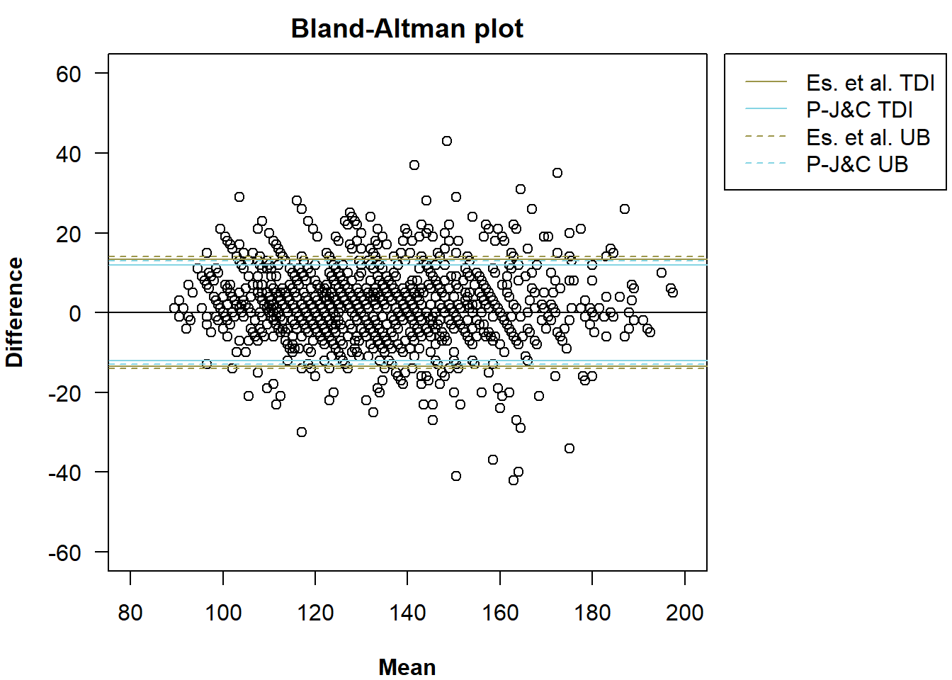
The colours of the lines can be changed with the argument
method.col.
plot(x, tdi = TRUE, ub = TRUE,
     method = c("es", "pe"), method.col = c("darkred", "darkolivegreen"),
     legend = TRUE, inset = c(-0.4, 0),
     xlim = c(80, 200), ylim = c(-60, 60))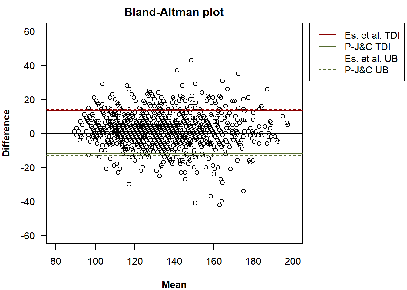
In the method of Perez-Jaume and Carrasco, up to eight UBs can be
computed. The one shown by default is the first one estimated from the
call of the function TDI() but it can be changed via the
argument ub.pc. Possible values are: p_db,
n_db, e_db, b_db,
p_cb, n_cb, e_cb and
b_cb. The bootstrap approach (differences or cluster) is
indicated with ‘’db’’ and ‘’cb’’ and the strategy (based on percentiles,
the normal distribution, the empirical method or the BC\(_a\)) is indicated with ‘’p’‘,’‘n’‘,’‘e’’
and ‘’b’’. If we want to add the UB computed with the cluster bootstrap
based on the normal distribution:
plot(x, tdi = TRUE, ub = TRUE, ub.pc = "n_cb",
     method = c("es", "pe"), method.col = c("darkred", "darkolivegreen"),
     legend = TRUE, inset = c(-0.4, 0),
     xlim = c(80, 200), ylim = c(-60, 60))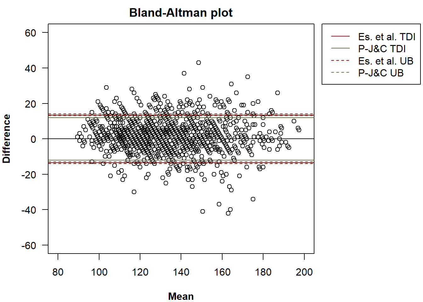
We can exclusively add the TDI estimates or the UBs.
plot(x, tdi = TRUE,
     method = c("es", "pe"), method.col = c("darkred", "darkolivegreen"),
     legend = TRUE, inset = c(-0.4, 0),
     xlim = c(80, 200), ylim = c(-60, 60))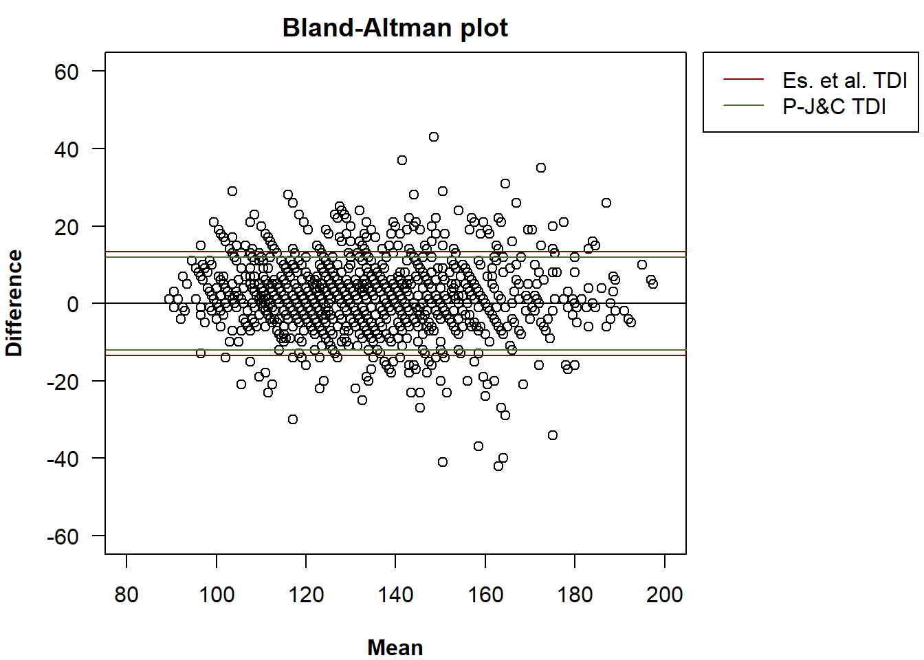
plot(x, ub = TRUE, ub.pc = "n_cb",
     method = c("es", "pe"), method.col = c("darkred", "darkolivegreen"),
     legend = TRUE, inset = c(-0.4, 0),
     xlim = c(80, 200), ylim = c(-60, 60))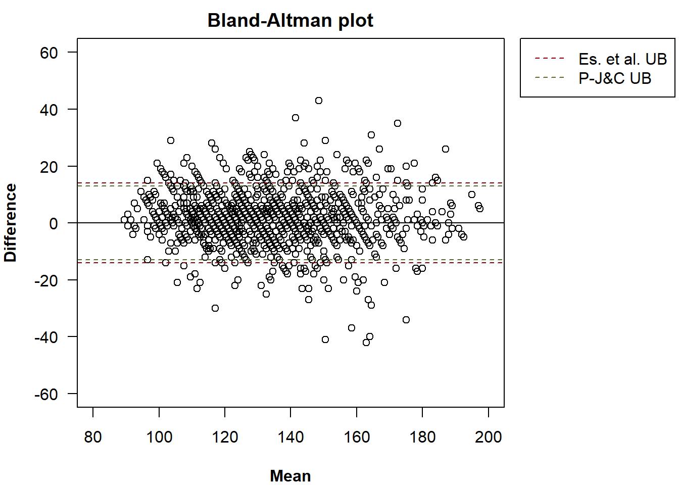
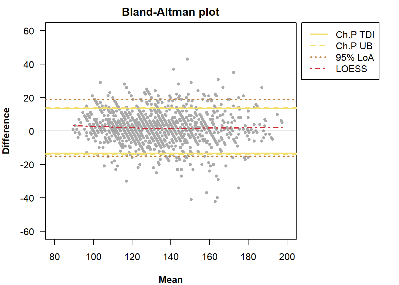
We can also add a locally estimated scatterplot smoothing (LOESS), otherwise referred to as LOESS curve, to the Bland-Altman plot, which facilitates the detection of systematic trends or non-constant bias. Adding this non-parametric smoothing curve aids in visually assessing whether, and how, agreement between raters varies across the range of values of the measurements.
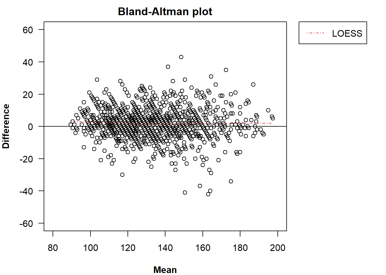
We can change the colour with the argument
loess.col.
plot(x, loess = TRUE, loess.col = "green",
     legend = TRUE, inset = c(-0.33, 0),
     xlim = c(80, 200), ylim = c(-60, 60))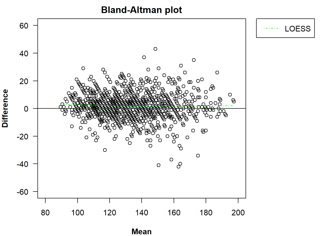
The smoothness parameter for loess.smooth() can be
modified via loess.span.
plot(x, loess = TRUE, loess.col = "green", loess.span = 2,
     legend = TRUE, inset = c(-0.33, 0),
     xlim = c(80, 200), ylim = c(-60, 60))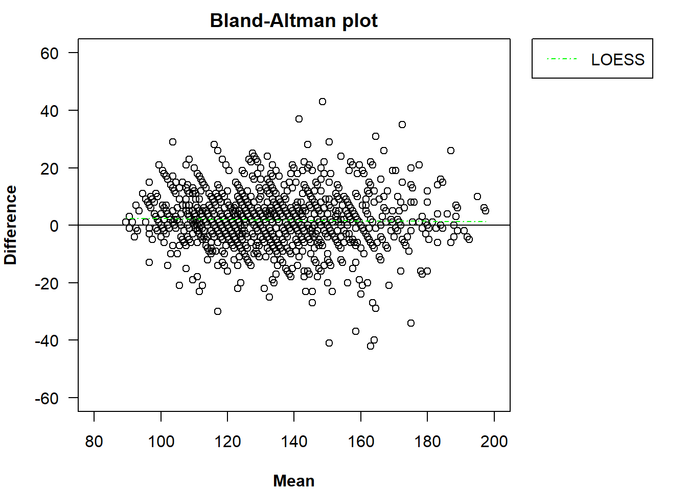
We can add more than one element to the plot.
plot(x, tdi = TRUE, ub = TRUE, method = "choudhary p",
     loa = TRUE, loess = TRUE,
     legend = TRUE, inset = c(-0.33, 0),
     xlim = c(80, 200), ylim = c(-60, 60))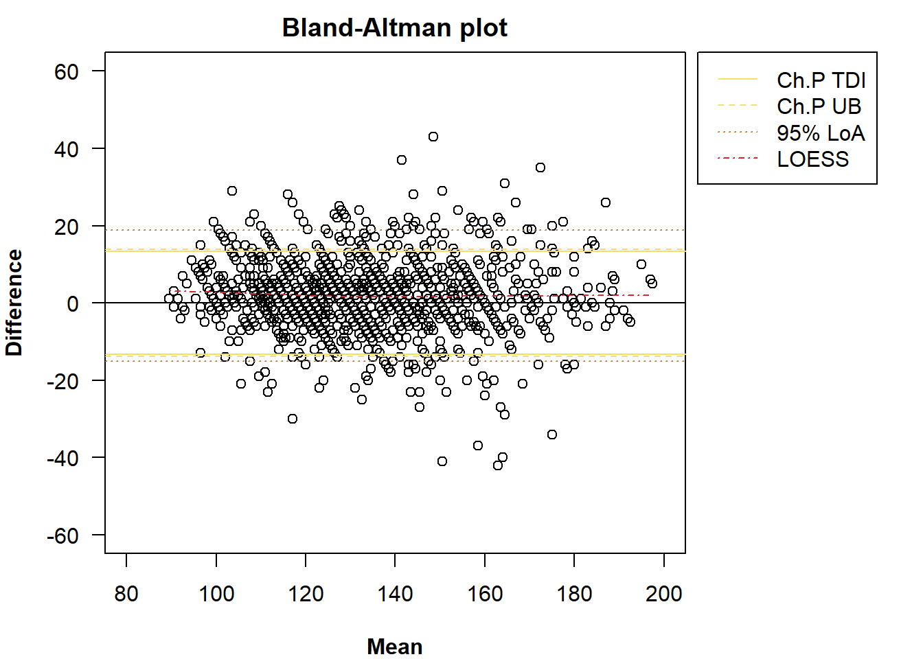
Finally, we can modify the line width of the TDI, UB, LoA lines and
LOESS curve with a 4-dimensional numerical vector passed to
lwd. A line width should be indicated for each
addendum.
plot(x, tdi = TRUE, ub = TRUE, method = "choudhary p",
     loa = TRUE, loess = TRUE,
     lwd = c(2, 2, 2, 2),
     legend = TRUE, inset = c(-0.33, 0),
     xlim = c(80, 200), ylim = c(-60, 60))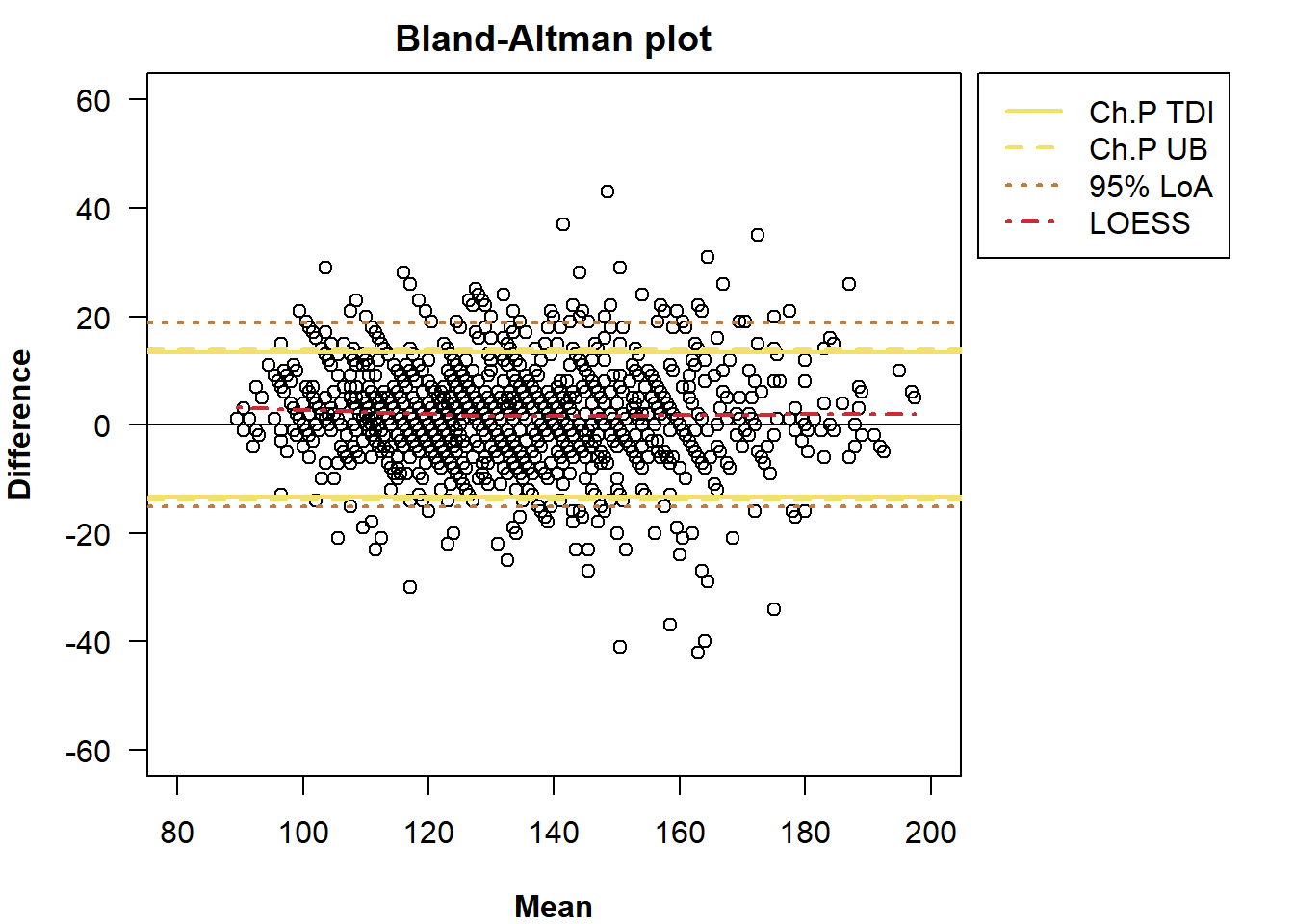
Other graphical parameters (to be passed to plot()) can
be modified with the ellipsis (...). For example, the
colour or symbol of the points.
plot(x, tdi = TRUE, ub = TRUE, method = "choudhary p",
     loa = TRUE, loess = TRUE,
     lwd = c(2, 2, 2, 2),
     legend = TRUE, inset = c(-0.33, 0),
     xlim = c(80, 200), ylim = c(-60, 60),
     col = "darkgrey", pch = 20)